The elementary error of physics that caused the global warming scare

— By Christopher Monckton of Brenchley

This will be a long posting, but it will not be found uninteresting.

Global warming on trial: Global warming goes on trial at 8.00 am this Wednesday, 21 March 2018, in Court 8 on the 19^th floor of the Federal Building at 450 Golden Gate Avenue, San Francisco. Court 8 is the largest of the courtrooms in the Federal District Court of Northern California. They’re clearly expecting a crowd. The 8 am start, rather than the usual 10 am, is because the judge in the case is an early bird. The judge: His Honour Judge William Haskell Alsup, who will preside over the coyly-titled “People of California” v. British Petroleum plc et al., is not to be underestimated. Judge Alsup, as the senior member of the Northern California Bench (he has been there for almost two decades), gets to pick the cases he likes the look of. He is no ordinary, custard-faced law graduate. Before he descended to the law (he wanted to help the civil rights movement), he earned a B.S. in engineering at Mississippi State University.

Don’t mess with me: His Honour Judge Alsup flourishing a  tract
by his mentor, the Supreme Court justice whom he once served as Clerk.

Six years ago, in an acrimonious hearing between Oracle and Google, the two Silicon-Valley giants were arguing about nine lines of computer code, which Oracle said Google had filched for its Android cellphone system. In preparation for the case, Oracle had tested 15 million lines of Android code, and had found that just nine lines – a subroutine known as rangeCheck – had been copied keystroke for keystroke. Oracle’s case was that these nine lines of code, though representing only 0.00006% of the Android software, were a crucial element in the system. Judge Alsup did not buy that argument.

Rumours gather about great men. In hushed tones, those who talk of Judge Alsup say he taught himself the Java programming language so that he could decide the rangeCheck case. In fact, he is not familiar with Java, but he does write computer code using qBasic, which used to be bundled free with MS-DOS. On the vast desk in his book-lined office sits a 2011-vintage Dell laptop, the only one he has that will still run qBasic. He has written programs for his ham-radio hobby, for the Mastermind board game, and for his wife’s bridge game.

The 18-year-old Bill Alsup at his
ham radio console in Mississippi:

This, then, is that rarest of creatures, a tech-savvy judge. And he has taken the very rare but commendable step of ordering both parties to answer nine scientific questions about climate change in preparation for what he has called a “tutorial” on the subject next Wednesday.

Hearing of this case, and of Bill Alsup’s starring role, I wondered what line of argument might convince a scientifically literate judge that the plaintiffs, two Californian cities who want the world’s five biggest oil corporations to pay them to adapt to rising sea level, that there is no cause for alarm about manmade global warming.

Judge Alsup might well be moved to dismiss the plaintiffs’ case provided that the defendants were able to establish definitively that fears of global warming had been very greatly exaggerated.

Two propositions: If the following two propositions were demonstrated, His Honor might decide – and all but a few irredentists would be compelled to agree – that global warming was not a problem and that the scare was over.

1. It can be proven that an elementary error of physics is the sole cause of alarm about global warming – elementary because otherwise non-climatologists might not grasp it.
2. It can be proven that, owing to that elementary error, current official mid-range estimates of equilibrium sensitivity to anthropogenic activity are at least twice what they should be.

Regular readers will know that my contributions here have been infrequent in the past year. The reason is that I have had the honor to lead a team of eminent climatological researchers who have been quietly but very busily investigating how much global warming we may cause, known as the “equilibrium-sensitivity” question.

We can now prove both points itemized above, and we have gone to more than customary lengths to confirm by multiple empirical methods what we originally demonstrated by a theoretical method. The half-dozen methods all cohere in the same ballpark.

Three days before His Honour posted up his list of questions on climate science, my team had submitted a paper on our result to a leading climatological journal (by convention, I am bound not to say which until publication).

The judge’s question: When I saw His Honour’s eighth question, “What are the main sources of heat that account for the incremental rise in temperature on Earth?”, I contacted my eight co-authors, who all agreed to submit an amicus curiae or “friend-of-the-court” brief.

Our reply: Our amicus brief, lodged for us by a good friend of the ever-valuable Heartland Institute, concludes with a respectful recommendation that the court should reject the plaintiffs’ case and that it should also order the oil corporations to meet their own costs in the case because their me-too public statements to the effect that global warming is a “problem” that requires to be addressed are based on the same elementary error as the plaintiffs’ case.

In effect, the oil corporations have invited legal actions such as this, wherefore they should pay the cost of their folly in accordance with the ancient legal principle volenti non fit injuria – if you stick your chin out and invite someone to hit it, don’t blub if someone hits it.

The judge has the right to accept or reject the brief, so we accompanied our brief with the usual short application requesting the court to accept it for filing. Since the rules of court require the brief to be lodged as an exhibit to the application, the brief stands part of the court papers in any event, has been sent to all parties, and is now publicly available on PACER, the Federal judiciary’s public-access database.

Therefore, I am at last free to reveal what we have discovered. There is indeed an elementary error of physics right at the heart of the models’ calculations of equilibrium sensitivity. After correcting that error, and on the generous assumption that official climatology has made no error other than that which we have exposed, global warming will not be 3.3 ± 1.2 K: it will be only 1.2 ± 0.15 K. We say we can prove it.

The proof: I shall now outline our proof. Let us begin with the abstract of the underlying paper. It is just 70 words long, for the error (though it has taken me a dozen years to run it to earth) really is stupendously elementary:

Abstract: In a dynamical system, even an unamplified input signal induces a response to any feedback. Hitherto, however, the large feedback response to emission temperature has been misattributed to warming from the naturally-occurring, non-condensing greenhouse gases. After correction, the theoretically-derived pre-industrial feedback fraction is demonstrated to cohere with the empirically-derived industrial-era value an order of magnitude below previous estimates, mandating reduction of projected Charney sensitivity from 3-3 ± 1.2 K to 1.2 ± 0.15 K.

Equations: To understand the argument that follows, we shall need three equations.

The zero-dimensional-model equation (1) says that equilibrium sensitivity or final warming ΔT_eq is the ratio of reference sensitivity or initial warming ΔT_ref to (1 – f ), where f is the feedback fraction, i.e., the fraction of ΔT_eq represented by the feedback response ΔT_(ref) to ΔT_ref. The entire difference between reference and equilibrium sensitivity is accounted for by the feedback response ΔT_(ref) (the bracketed subscript indicates a feedback response).

ΔT_eq = ΔT_ref / (1 – f ).    (1)

The zero-dimensional model is not explicitly used in general-circulation models. However, it is the simplest expression of the difference between reference sensitivity before accounting for feedback and equilibrium sensitivity after accounting for feedback. Eq. (1), a simplified form of the feedback-amplification equation that originated in electronic network analysis, is of general application when deriving the feedback responses in all dynamical systems upon which feedbacks bear. The models must necessarily reflect it.

Eq. (1) is used diagnostically not only to derive equilibrium sensitivity (i.e., final warming) from official inputs but also to derive the equilibrium sensitivity that the models would be expected to predict if the inputs (such as the feedback fraction f ) were varied. We conducted a careful calibration exercise to confirm that the official reference sensitivity and the official interval of the feedback fraction, when input to Eq. (1), indeed yield the official interval of equilibrium sensitivity.

The feedback-fraction equation (2): If the reference sensitivity ΔT_ref and the equilibrium sensitivity ΔT_eq are specified, the feedback fraction f is found by rearranging (1) as (2):

f  = 1 – ΔT_ref / ΔT_eq.    (2)

The reference-sensitivity equation (3): Reference sensitivity ΔT_ref is the product of a radiative forcing ΔQ₀, in Watts per square metre, and the Planck reference-sensitivity parameter λ₀, in Kelvin per Watt per square metre.

ΔT_ref = λ₀ ΔQ₀.    (3)

The Planck parameter λ₀ is currently estimated at about 0.3125, or 3.2^–1 K W^–1 m² (Soden & Held 2006; Bony 2006, Appendix A; IPCC 2007, p. 631 fn.). The CO₂ radiative forcing ΔQ₀ is 3.5 W m^–2 (Andrews 2012). Therefore, from Eq. (3), reference sensitivity ΔT_ref to doubled CO₂ concentration is about 1.1 K.

The “natural greenhouse effect” is not 32 K: The difference of 32 K between natural temperature T_N (= 287.6 K) in 1850 and emission temperature T_E (= 255.4 K) without greenhouse gases or temperature feedbacks was hitherto imagined to comprise 8 K (25%) base warming ΔT_B directly forced by the naturally-occurring, non-condensing greenhouse gases and a 24 K (75%) feedback response ΔT_(B) to ΔT_B, implying a pre-industrial feedback fraction f ≈ 24 / 32 = 0.75 (Lacis et al., 2010).

Similarly, the CMIP3/5 models’ mid-range reference sensitivity ΔT_S (= 3.5 x 0.3125 = 1.1 K) and Charney sensitivity ΔT (= 3.3 K) (Charney sensitivity is equilibrium sensitivity to doubled CO₂), imply a feedback fraction f = 1 – 1.1 / 3.3 = 0.67 (Eq. 2) in the industrial era.

The error: However, climatologists had made the grave error of not realizing that emission temperature T_E (= 255 K) itself induces a substantial feedback. To correct that long-standing error, we illustratively assumed that the feedback fractions f in response to T_E and to ΔT_B were identical. Then we derived f simply by replacing the delta values ΔT_ref, ΔT_eq in (2) with the underlying entire quantities T_ref, T_eq, setting T_ref = T_E + ΔT_B, and T_eq = T_N (Eq. 4),

f  = 1 –T_ref / T_eq = 1 – (T_E + ΔT_B) / T_N

= 1 – (255.4 + 8) / 287.6 = 0.08.    (4)

Contrast this true pre-industrial value f = 0.08 with the CMIP5 models’ current mid-range estimate f = 1 – 1.1 / 3.3 = 0.67 (Eq. 2), and with the f = 0.75 applied by Lacis et al. (2010) not only to the 32 K “entire natural greenhouse effect” but also to “current climate”.

Verification: We took no small trouble to verify by multiple empirical methods the result derived by the theoretical method in Eq. (4).

Test 1: IPCC’s best estimate (IPCC, 2013, fig. SPM.5) is that some 2.29 W m^–2 of net anthropogenic forcing arose in the industrial era to 2011. The product of that value and the Planck parameter is the 0.72 K reference warming (Eq. 3).

However, 0.76 K warming was observed (taken as the linear trend on the HadCRUT4 monthly global mean surface temperature anomalies, 1850-2011).

Therefore, the industrial-era feedback fraction f is equal to 1 – 0.72 / 0.76. or 0.05 (Eq. 2). That is close to the pre-industrial value f = 0.08: but it is an order of magnitude (i.e., approximately tenfold) below the models’ 0.67 or Lacis’ 0.75.

There is little chance that some feedbacks had not fully acted. The feedbacks listed in IPCC (2013, p. 818, table 9.5) as being relevant to the derivation of equilibrium sensitivity are described by IPCC (2013, p. 128, Fig. 1.2) as having the following durations: Water vapour and lapse-rate feedback hours; Cloud feedback days; Surface albedo feedback years.

The new headline Charney sensitivity: Thus, Charney sensitivity is not 1.1 / (1 – 0.67) = 3.3 K (Eq. 1), the CMIP5 models’ imagined mid-range estimate (Andrews 2012). Instead, whether f = 0.05 or 0.08, Charney sensitivity ΔT_eq = 1.1 / (1 – f ) is 1.2 K (Eq. 1). That new headline value is far too small to worry about.

Test 2: We sourced mainstream estimates of net anthropogenic forcing over ten different periods in the industrial era, converting each to reference sensitivity using Eq. (3) and then finding the feedback fraction f for each period using Eq. (2).

The mean of the ten values of f was 0.12, somewhat higher than the value 0.05 based on IPCC’s mid-range estimate of 2.29 W m^–2 net anthropogenic forcing in the industrial era. The difference was driven by three high-end outliers in our table of ten results. Be that as it may, Charney sensitivity for f = 0.12 is only 1.25 K.

Test 3: We checked how much global warming had occurred since 1950, when IPCC says our influence on climate became detectable. The CMIP5 mid-range prediction of Charney sensitivity, at 3.3 K, is about equal to the original mid-range prediction of 21^st-century global warming derivable from IPCC (1990, p. xiv), where 1.8 K warming compared with the pre-industrial era [equivalent to 1.35 K warming compared with 1990] is predicted for the 40-year period 1991-2030, giving a centennial warming rate of 1.35 / (40 / 100) = 3.3 K.

This coincidence of values allowed us to compare the 1.2 K Charney sensitivity derived from f on (0.05, 0.12) in Eq. (4) with the least-squares linear-regression trend on the HadCRUT4 monthly global mean surface temperature anomalies over the 68 years 1950-2017. Sure enough, the centennial-equivalent warming was 1.2 K/century:

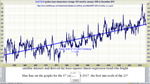
The centennial-equivalent warming rate from 1950-2017 was 1.2 K/century

Test 4: We verified that the centennial-equivalent warming rate in the first 17 years (one-sixth) of the 21^st century was not significantly greater than the rate since 1950. We averaged the monthly global mean surface and lower-troposphere temperature anomalies from the HadCRUT4 terrestrial and UAH satellite datasets and derived the least-squares linear-regression trend (the bright blue line on the graph below).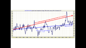

The satellite data were included because they cover a five-mile-high slab of the atmosphere immediately above the surface, and have a coverage greater than the terrestrial measurements. The trend was found to be 0.22 K, equivalent to 1.3 K/century:

Test 5: To confirm that we had understood feedback theory correctly, one of my distinguished co-authors, a hands-on electronics engineer, heard of our result and built a test rig in which we were able to specify the input signal (i.e., emission temperature T_E) as a voltage, and also the direct-gain factor μ to allow for direct natural or anthropogenic forcings, and the feedback fraction β (we were using the more precise form of Eq. 1 that is usual in electronic network analysis). Then it was a simple matter directly to measure the output signal (i.e., equilibrium sensitivity ΔT_eq).

The most crucial of the many experiments we ran on this rig was to set μ to unity, implying no greenhouse forcing at all. We set the feedback fraction β to a non-zero value and then verified that the output signal exceeded the input signal by the expected margin. Not at all to our surprise, it did. This experiment proved that emission temperature, on its own, induced a feedback response that climatology had hitherto overlooked.

This is where the elementary error made by climatologists for half a century has had its devastating effect. Look again at Eq. (1). The input signal is altogether absent. Although it is acceptable to use Eq. (1) to derive equilibrium sensitivities from reference sensitivities, the mistake made by the modellers was to assume, as Lacis et al. (2010) and many others had assumed, that the entire difference of 32 K between the natural temperature T_N in 1850 and the emission temperature T_E was accounted for by the natural greenhouse effect, comprising a direct greenhouse warming ΔT_B = 8 K and a very large feedback reponse ΔT_(B) = 24 K to ΔT_B.

However, in truth – this is the crucial point – the emission temperature T_E (= 255 K), even in the absence of any greenhouse gases, induces a large feedback response ΔT_E. This feedback response to the input signal is entirely uncontroversial in electronic network analysis and in control theory generally, but we have not been able to find any acknowledgement in climatology that it exists.

Just as Lacis (2010) did, the modellers assumed that the industrial-era feedback fraction must be every bit as large as the pre-industrial feedback fraction that they had erroneously inflated by adding the large feedback response induced by emission temperature to the small feedback response induced by the presence of the naturally-occurring greenhouse gases.

It was that assumption that led the modellers to assume that there must be some very strongly positive feedbacks, chief among which was the water-vapour feedback. However, although the Clausius-Clapeyron relation indicates that the space occupied by the atmosphere can carry near-exponentially more water vapour as it warms, there is nothing to say that it must.

Suppose there were a water-vapour feedback anything like as large as that which the models have assumed (and they have assumed a very large feedback only because they are trying to explain the large but fictitious feedback fraction consequent upon their erroneous assumption that emission temperature of 255 K somehow induces no feedback response at all, while the next 8 K of warming magically induces a 24 K feedback response). In that event, atmospheric dynamics requires that there must be a tropical mid-troposphere “hot spot” [I had the honour to name it], where the warming rate should be twice or thrice that at the tropical surface. However, the “hot spot” is not observed in reality (see below), except in one suspect dataset that Dr Fred Singer scrutinized some years ago and determined to be defective.

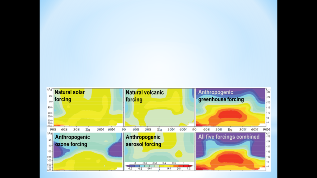
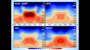
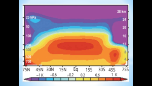
Models predict the tropical mid-troposphere “hot spot” (top, IPCC 2007, citing Santer 2003; left, Lee et al., 2008; right, Karl et al., 2006).

However, the “hot spot” is not observed in reality (see below). Our result shows why not. The “hot spot” is an artefact of the modellers’ error in misallocating the substantial feedback response induced by emission temperature by adding it to the very small feedback response induced by the naturally-occurring greenhouse gases.

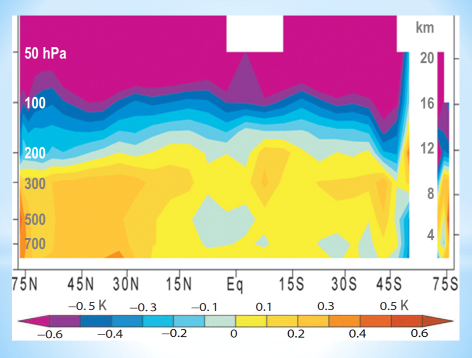
The model-predicted “hot spot” is not observed in reality (Karl et al., 2006).

Test 6: Even after we had built and operated our own test rig – as far as we know, this is the first time anyone has tried to test climatological feedback theory empirically rather than simply modelling it – we were not satisfied that anything other than tests performed under rigorous conditions at a government laboratory would be found widely acceptable.

Accordingly, based on the results of our in-house test rig, we drew up a more sophisticated specification for a new rig, together with four test groups comprising 23 sets of three quantities – the input signal, the direct-gain factor and the feedback fraction. Armed with the specification, I commissioned a government laboratory to carry out the experiments.

However, a problem at once arose – indeed, it was a problem with which our own engineer had wrestled. So very small were the feedback responses predicted by long-established control theory that even the presence of the operator in the same room as the test rig tended to bias the results.

Accordingly, I worked for months with a patient and amiable scientist at the government laboratory. Eventually, by somewhat altering the initial-state values specified for the 23 tests, I was able to give the scientist values that would yield results to the required precision but without loss of experimental integrity.

In due course the laboratory reported, and the results of all 23 tests – to within one-tenth of a Kelvin – were exactly as we had been able to predict theoretically. Again, the most important results were for the group of tests in which the direct-gain factor was set to unity, so that we could reassure ourselves that control theory was correct in predicting that, in the presence of a non-zero feedback fraction, even an unamplified input signal would induce a feedback response that would either amplify or attenuate it.

Another snag arose. When I had originally approached the laboratory, I had not mentioned that the research had anything to do with climate change, because all I wanted to do was to establish that we had understood the relevant control theory correctly.

When the laboratory reported, I sent it a copy of our draft paper, in which the lab results were mentioned. The laboratory panicked and said we were not allowed to use its report.

However, I had written into the contract a term to the effect that we intended to include the laboratory’s results, and a discussion of them, in an academic paper. A compromise was reached, by which we are free to include the laboratory’s results in our paper, as long as we do not mention either the name of the laboratory or the name of the scientist there who built and ran the high-specification rig for us.

The laboratory also kindly confirmed that we had represented its results fairly in our paper and had drawn justifiable conclusions from them. Furthermore, much to our pleasure, it promoted the scientist who had assisted us. He wrote us a charming letter to say that he had not allowed, and would not allow, politics to intrude into the work he had carried out for us.

With these results from a national laboratory (we cannot even mention which country it was in) we were at last content that we had established our conclusion with sufficient rigor.

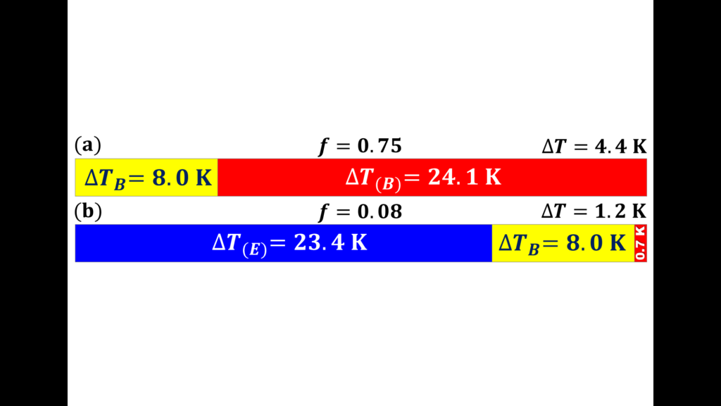
The true picture: How should the 32 K difference between emission temperature and natural temperature be apportioned? Approximately 23.4 K of the 32 K is the feedback response to emission temperature; 8 K is the directly-forced warming from the presence of the natural greenhouse gases; and just 0.7 K is feedback response to that 8 K warming (panel b):

• Erroneous apportionment of the 32 K difference between natural temperature in 1850 and emission temperature in the absence of any greenhouse gases, given in Lacis et al. (2010).
• Corrected apportionment of the 32 K, allowing for the feedback response (blue) to emission temperature; the directly-forced warming from the naturally-occurring, non-condensing greenhouse gases (yellow); and the feedback response to that greenhouse warming (red).

Looking at it the other way about, if the feedback fraction were really as large as the 0.75 imagined by Lacis et al. (2010), then the Earth’s emission temperature of 255.4 K would induce a feedback response of 766.2 K, and the 8 K greenhouse warming would induce a feedback response of 24 K, so that the pre-industrial or natural temperature in 1850 would be 255.4 + 766.2 + 8 + 24 ≈ 1054 K, about three and a half times the true value of 287.6 K.

We also considered whether non-linearities in individual feedbacks might vitiate our result. However, to obtain even the 1.5 K minimum Charney sensitivity predicted by IPCC one would need to multiply at least fivefold the empirically-derived industrial-era feedback fraction f = 0.05.

The reason why even a very large nonlinearity in the feedback sum and consequently in the feedback fraction makes little difference to equilibrium sensitivities is that the curve of equilibrium sensitivities in the presence of various feedback factors is a rectangular hyperbola (see below). Our result shows that the sensitivity calculation is not done, as now, rather close to the singularity at f = 1 (note in passing that for f > 1 Eq. (1) predicts cooling); instead, it is done at the left-hand end of the curve, where the sensitivity increases very slowly with f:

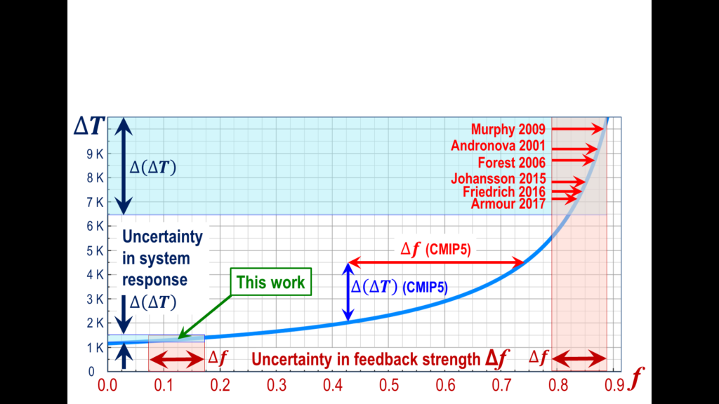
The rectangular-hyperbolic curve of Charney sensitivities in response to feedback fractions f,
showing current predictions compared with the corrected result.

The outcome of the case: What will His Honour make of all this? My guess is that he will allow our amicus brief to be filed. With his engineering background, he will have no difficulty in understanding why we say that the notion of catastrophic rather than moderate global warming is rooted in the elementary physical error we have discovered.

Therefore, we hope His Honour will ask all parties to provide formal responses to our brief. On any view, it plainly raises a serious question about whether global warming matters at all – a question that strikes right to the heart not only of the case before him but of numerous other such cases now arising in several jurisdictions – and showing some evidence of careful co-ordination.

The parties will not be able to dismiss our result lightly. To refute it, they would have to show that our pre-industrial feedback fraction f = 0.08, obtained by theoretical means rooted in mainstream control theory, is incorrect; that our industrial-era value f = 0.05, obtained empirically from IPCC’s estimate of the net anthropogenic forcing to date and from the HadCRUT4 temperature record, is also incorrect; that our campaign of ten empirical calculations giving a mean feedback fraction f = 0.12, is incorrect; that the rate of observed warming over the past 68 years is either incorrect or irrelevant; that the rate of observed warming this century to date is also either incorrect or irrelevant; that the results from our test rig are inapplicable; that the results from a government laboratory are likewise inapplicable; and, above all, that it is justifiable to assume that control theory is wrong and that, per impossibile, 255.4 K of emission temperature generates no feedback at all, while the next 8 K of warming suddenly causes 24 K of feedback, as if by magic.

We do not believe in magic.

Conclusion: The anthropogenic global warming we can now expect will be small, slow, harmless, and even net-beneficial. It is only going to be about 1.2 K this century, or 1.2 K per CO₂ doubling. If the parties are not able to demonstrate that we are wrong, and if His Honour accepts that we have proven the result set out publicly and in detail here for the first time, then the global warming scare was indeed based on a strikingly elementary error of physics.

The avowedly alarmist position too hastily adopted by governments and international bureaucratic entities has caused the most egregious misallocation of resources in history.

Ladies and gentlemen, we call time on a 50-year-old scam, in which a small number of corrupt and politicized scientists, paid for by scientifically-illiterate governments panicked by questionable lobby-groups funded by dubious billionaires and foreign governments intent on doing down the West, and egged on by the inept and increasingly totalitarian news media, have conspired to perpetrate a single falsehood: that the science was settled.

Well, it wasn’t.

Views: 1123